I had my genome sequenced, and got back two files: a pair of gzipped FASTQs, about 150 GB, holding a few billion short DNA reads. That is the raw output of a sequencer — essentially a giant pile of 150-letter fragments with no idea where in the genome each one belongs. Turning that into something you can actually read — here is where you differ from the reference human genome, and here is what those differences might mean — is a real computational pipeline.
This is the story of building that pipeline for a single person, me, running it on Google Cloud Batch, and a fun detour at the end: profiling the oral microbiome from the reads that didn’t look human.
What “analyzing a genome” actually means Link to heading
The reference human genome (I use GATK’s GRCh38 build) is a fixed 3-billion-letter string. Your genome is 99.9% identical to it. All the interesting information is in the differences: single-letter swaps (SNVs), small insertions and deletions (indels), large rearrangements (structural variants), and stretches that are duplicated or missing (copy-number variants). The job of the pipeline is to find those differences reliably and then annotate them — cross-reference each one against databases that say this variant sits in this gene and is predicted to break the protein, or this one is benign and half the population carries it.
Rather than reinvent any of this, I stood on nf-core/sarek,
a mature, community-maintained Nextflow pipeline for germline
and somatic variant calling. Pinned to v3.9.0 for reproducibility. Sarek knows how to
orchestrate the dozens of tools involved; my job was to configure it for one healthy
person’s genome and make it run economically in the cloud.
The pipeline, from FASTQ to annotated variants Link to heading
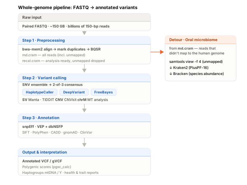
The whole pipeline at a glance: a three-step spine from raw reads to annotated variants, with the microbiome detour branching off the md.cram from Step 1.
I split the run into three checkpointed steps, each a thin wrapper around sarek that
shares a run name so Nextflow can -resume from cache if something fails partway:
Step 1 — Preprocessing. Trim and split the raw FASTQs, align every read to GRCh38
with bwa-mem2, mark PCR duplicates, and run base-quality score recalibration (BQSR).
The output is an analysis-ready recalibrated
CRAM — the reads, now placed on
the genome and cleaned up.
Step 2 — Variant calling. This is where the biology appears. For small variants I
run an ensemble of three callers — GATK HaplotypeCaller, Google’s DeepVariant, and
FreeBayes — because they disagree at the margins and the agreement between them is a
useful confidence signal. Sarek then normalizes all three with bcftools norm (so the
same variant is written the same way) and builds a 2-of-3 consensus: a
high-confidence set of variants that at least two independent callers found. Structural
variants come from Manta and TIDDIT, copy-number from CNVkit, and there’s a dedicated
mitochondrial analysis on the side.
tools: haplotypecaller,freebayes,deepvariant,manta,tiddit,cnvkit
run_mt_analysis: true
concatenate_vcfs: true
normalize_vcfs: true
snv_consensus_calling: 2   # keep variants seen by ≥2 of the 3 SNV callers
One decision worth calling out: I deliberately excluded all the somatic callers (Mutect2, ASCAT, Control-FREEC). Those exist to compare a tumor against matched normal tissue and find cancer mutations. I have one germline sample — one person, no tumor — so those tools have nothing to compare against and would only add cost and noise.
Step 3 — Annotation. Run the variants through snpEff and VEP (Ensembl’s
Variant Effect Predictor), plus the dbNSFP plugin, which attaches a wall of
functional-prediction scores to each coding variant: SIFT, PolyPhen, REVEL, CADD,
gnomAD population frequencies, ClinVar clinical significance, and more. This is the step
that turns a coordinate like chr7:117559590 A>G into “in CFTR, predicted damaging,
present in ClinVar.”
The whole thing runs from a small orchestrator VM that just launches the Nextflow run; all the heavy compute happens out on Batch.
Making Google Cloud Batch fast and cheap Link to heading
This is the part I found most interesting as an engineering problem. The pipeline runs dozens of different tasks with very different appetites — some want many cores, some want lots of memory, some are quick and cheap — and matching each one to the right machine is what keeps the run fast and the bill small.
Spot VMs everywhere Link to heading
The single biggest lever is Spot VMs — Google’s preemptible instances, at roughly a 60–90% discount. The risk is that Google can reclaim them mid-task. Nextflow handles this gracefully if you tell it to retry on preemption:
google.batch.spot = true
google.batch.maxSpotAttempts = 5

process {
  // retry only transient / OOM / preemption exit codes; fail fast on real errors
  errorStrategy = { task.exitStatus in ((130..145) + [104, 50001, 50002, 50003, 50006]) ? 'retry' : 'finish' }
  maxRetries = 5
}
The subtlety is in that errorStrategy. I only want to retry on the codes that mean
“the machine went away” or “we ran out of memory” — not on a genuine tool error, which
retrying would just repeat five times before failing anyway. So preemption and OOM
codes retry; everything else fails fast so I hear about it immediately.
Sizing each process from measured traces, not guesses Link to heading
Nextflow lets you attach different machine specs to each process by name. The naive approach is to give everything a big machine. The economical approach is to look at what each step actually used and size to that. Nextflow emits an execution trace with peak RSS, CPU utilization, and runtime per task, so after a first run I went through it and pinned machine types to reality. The config reads like a set of field notes:
withName:BWAMEM2_MEM {
  machineType = 'n2-custom-12-49152'   // 12 vCPU / 48 GB: measured ~12.6 cores, 27 GB peak
  cpus = 12; memory = 48.GB; disk = '150 GB'
}

withName:DEEPVARIANT_RUNDEEPVARIANT {
  machineType = 'n2-custom-16-32768'   // measured 18.8 GB peak, ~12.8 cores
  cpus = 16; memory = 30.GB; disk = '150 GB'
}

withName:GATK4_HAPLOTYPECALLER {
  machineType = 'n2-highcpu-8'         // 8 cpu fully used (measured 796%); peak RSS 4.2 GB
  cpus = 8; memory = 6.GB; disk = '75 GB'
}
Those comments are the whole point. n2-custom-12-49152 isn’t a stock machine shape —
it’s a custom VM with exactly 12 vCPUs and 48 GB of RAM, because the trace said
BWA-MEM2 peaks around 12.6 cores and 27 GB, and paying for a standard 16-core box would
waste a third of it. VEP is the nicest example: dbNSFP is a ~30 GB database, and the
instinct is to give the VM enough RAM to hold it. But VEP streams it via tabix, so peak
memory is only 2.3 GB — it wants CPUs (--fork 16), not RAM. Reading the trace saved a
64 GB machine there.
Where I didn’t pin a machine type, Google Batch auto-sizes the VM from the task’s
declared cpus/memory, so sarek’s own resource labels are still honored. A global cap
keeps any single task from requesting something absurd:
resourceLimits = [ cpus: 64, memory: 256.GB, time: 240.h ]
Scatter width and private networking Link to heading
Two more settings matter. split_fastq chops the input FASTQs into chunks so alignment
fans out across many VMs in parallel instead of grinding through one huge file, and
nucleotides_per_second controls how finely variant calling is scattered across genomic
intervals. Both trade a bit of scheduling overhead for a lot of parallelism.
And everything runs on private networking — usePrivateAddress = true, no external
IPs — with Fusion and Wave
disabled. Batch tasks read and write directly to a Google Cloud Storage bucket; the
reference genome, the work directory, and all results live in GCS, so the VMs are
ephemeral and hold no state.
Reading the output: from variants to answers Link to heading
The pipeline’s real output is a stack of files in a small zoo of bioinformatics formats, each a stage in the same story. FASTQ is the raw reads; BAM and CRAM are those reads aligned to the genome (CRAM is BAM with reference-based compression, roughly half the size); a VCF lists the variants; and a gVCF is a VCF that records a call at every position — including the ~99% where I match the reference — not just the sites where I differ. That last distinction turns out to matter more than it sounds.
A VCF full of coordinates isn’t an answer to anything by itself. Three things I do with it:
Polygenic scores. I ported a pgsc/ module that runs
pgsc_calc over the whole
PGS Catalog — thousands of published scores for traits and
disease risk — with genetic-ancestry adjustment, so each score comes back as a
percentile against the most-similar reference population rather than an
uninterpretable weighted sum. The catch that ate the most time: pgsc_calc expects
array-style data where every scored site has a genotype, but a variant-only VCF omits
every homozygous-reference site, so most scoring sites look “missing.” The fix is to
project the gVCF onto the scoring positions and write explicit 0/0 records where I match
the reference — which took a pilot’s match rate from a would-be failure to 99.8%. That’s
why the gVCF, not the variant VCF, is the input.
Haplogroups — deep maternal and paternal ancestry. Two small pieces of the genome are
inherited almost unchanged down a single line: mitochondrial DNA (chrM) passes from mother
to child, and the Y chromosome (chrY) from father to son. A tiny Batch job
(haplogroup_bams.sh) slices the chrM reads — and the chrY reads, when there’s real
coverage — into their own BAM files, which upload straight to
YFull for maternal (mtDNA) and paternal (Y) haplogroup placement
on the human tree. Same lineages the consumer ancestry tests report, but called from
full-depth whole-genome data.
Literature-linked health and trait interpretation. The consumer-genetics tools take a VCF directly now: hand the annotated VCF to Genetic Genie and it cross-references each variant against the published literature and hands back a browsable report. For digging into a single SNP, Genetic Lifehacks is a good place to read the actual studies.
A bonus: the oral microbiome hiding in the reads Link to heading
Here’s the detour I enjoyed most. My sample was a saliva/buccal swab. When you sequence saliva and align it to the human genome, a few percent of the reads don’t map — they aren’t human. Some of that is contamination and sequencing artifact, but a lot of it is real: bacteria, fungi, and viruses living in your mouth, sequenced right alongside your own DNA. The oral microbiome, for free, riding in the off-target reads.
So I built a small companion job to profile it. The workflow:
- Take the reads that failed to align (
samtools view -f 4, the unmapped flag). - Classify each one taxonomically with Kraken2 against the PlusPF-16 database (bacteria, archaea, fungi, protozoa, viruses).
- Re-estimate species-level abundances with Bracken.
samtools view -u -f 4 --reference ref.fasta -@ 8 md.cram \
  | samtools collate -u -O -@ 8 - /tmp/coltmp \
  | samtools fastq -@ 8 -1 unmapped_R1.fq.gz -2 unmapped_R2.fq.gz -s /dev/null -0 /dev/null -

kraken2 --db db --threads 8 --paired --gzip-compressed \
  unmapped_R1.fq.gz unmapped_R2.fq.gz \
  --report kraken_report.txt --output kraken_output.txt

bracken -d db -i kraken_report.txt -o bracken_species.txt -r 150 -l S
There was one non-obvious trap. Sarek produces two CRAM files: the recalibrated one
(recal.cram) and the markduplicates one (md.cram). It’s tempting to reach for the
final, “best” recalibrated file — but BQSR runs over genomic intervals that exclude
unmapped reads, so recal.cram has often dropped exactly the reads I need. The
microbiome lives in md.cram, the earlier file that still contains the complete read
set. Using the wrong input would have silently thrown away the entire signal.
This job doesn’t need Nextflow at all — it’s a single self-contained Google Batch job,
submitted with a Python-rendered job spec, running on an n2-highmem-8 because the
Kraken2 database has to sit in RAM during classification. Same cloud primitives,
much smaller scope.
Kraken2 is a general-purpose classifier, not a clinical instrument, so the honest caveat is that low-abundance hits in off-target WGS reads are frequently contamination or misclassification — I trust the dominant, biologically plausible taxa and treat the long tail as noise. But the dominant taxa in a saliva sample really are the usual suspects of the oral microbiome, which is a genuinely satisfying thing to see fall out of a genome sequencing run for free.
What I took away Link to heading
Three things stuck with me. First, the modern nf-core pipelines are extraordinary — a few YAML files and I have an ensemble variant-calling workflow that would have been a PhD’s worth of plumbing a decade ago. Second, cloud batch is at its best when you treat the execution trace as a design document: nearly every machine type in my config is justified by a measured number, and that discipline is where the cost savings actually live. And third, the most fun result — the oral microbiome — was sitting in the reads I would otherwise have thrown away. Data you already have is often more interesting than it looks.